<?xml version="1.0" encoding="utf-8"?>
<feed xmlns="http://www.w3.org/2005/Atom">
  <title>Yash Bitla</title>
  <link href="https://yashbitla.com/feed.xml" rel="self"/>
  <link href="https://yashbitla.com/"/>
  <id>https://yashbitla.com/</id>
  <updated>2026-10-09T00:00:00Z</updated>
  <author><name>Yash Bitla</name></author>
  
  <entry>
    <title>My object detector was too slow for live video. So I stopped waiting for it.</title>
    <link href="https://yashbitla.com/blog/stopped-waiting-for-the-detector/"/>
    <id>https://yashbitla.com/blog/stopped-waiting-for-the-detector/</id>
    <updated>2026-10-09T00:00:00Z</updated>
    <summary>A tracker that waits for a slow detector shows boxes that are 100 ms late. Running the detector in the background, with optical flow in between, cut that to 5 ms and scored higher.</summary>
    <content type="html"><p>A camera at 30 frames a second gives you a new frame every 33 ms. The object detector I wanted to use takes about 80 ms on my laptop CPU. So by the time it finishes one frame, the camera has moved on by two more.</p>
<p>Most tracking code ignores this. It runs the detector on every frame and assumes the detector keeps up. On recorded video that is fine, because the video waits. On a live stream, the world does not wait, and the boxes you draw are for where people were, not where they are.</p>
<p>I built <a href="https://github.com/yash-bitla/leantrack">leantrack</a> to answer one question: if the detector is a limited resource, when should it run, and what does each choice cost in accuracy?</p>
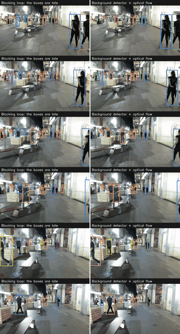
<p><img alt="Two views of the same street. On the left the boxes trail behind the people. On the right they stay on them." src="/img/leantrack-demo.gif" /></p>
<p>On the left, the loop waits for the detector, so the boxes are behind the people. On the right, the detector runs in the background and the boxes stay on them. Same detector, same video.</p>
<h2>The setup</h2>
<p>A tracker does two jobs. The <strong>detector</strong> finds people in one frame. The <strong>tracker</strong> connects those detections across frames, so that person 7 stays person 7.</p>
<ul>
<li><strong>Data:</strong> the MOT17 training set, seven street sequences.</li>
<li><strong>Detector:</strong> YOLOX-s through ONNX Runtime, on the CPU of an Apple M3 Pro.</li>
<li><strong>Metric:</strong> HOTA, which runs from 0 to 100 and rewards both finding people and keeping their identities.</li>
</ul>
<p>Two cautions before any numbers. First, my detector has general-purpose weights and was never trained on this dataset, so the absolute scores are low. The comparisons between configurations are the result. Second, I wrote the tracker core myself, so I checked it against a known implementation first: on the same detections it scores 47.11 HOTA against 47.32 for BoxMOT's ByteTrack. Close enough that the experiments after it mean something.</p>
<h2>First idea: run the detector less often</h2>
<p>The obvious move is to run the detector on every Nth frame and let the tracker predict the frames in between.</p>
<table>
<thead>
<tr>
<th>Detector runs on</th>
<th style="text-align: right;">Mean time per frame</th>
<th style="text-align: right;">HOTA</th>
</tr>
</thead>
<tbody>
<tr>
<td>Every frame</td>
<td style="text-align: right;">79.8 ms</td>
<td style="text-align: right;">37.5</td>
</tr>
<tr>
<td>Every 3rd frame</td>
<td style="text-align: right;">26.7 ms</td>
<td style="text-align: right;">36.0</td>
</tr>
<tr>
<td>Every 5th frame</td>
<td style="text-align: right;">16.1 ms</td>
<td style="text-align: right;">33.0</td>
</tr>
<tr>
<td>Every 10th frame</td>
<td style="text-align: right;">8.1 ms</td>
<td style="text-align: right;">28.9</td>
</tr>
</tbody>
</table>
<p>Skipping two frames out of three cuts the mean time by 67% and costs 1.5 points. That is a good trade. Past that, accuracy falls quickly.</p>
<p>There is a catch in this table that the mean hides. The slowest frames did not get faster: the 99th percentile stayed near 80 ms at every interval. A frame that runs the detector costs what it always cost. A fixed interval improves your average and does nothing for your worst case.</p>
<h2>Second idea: watch the pixels between detector runs</h2>
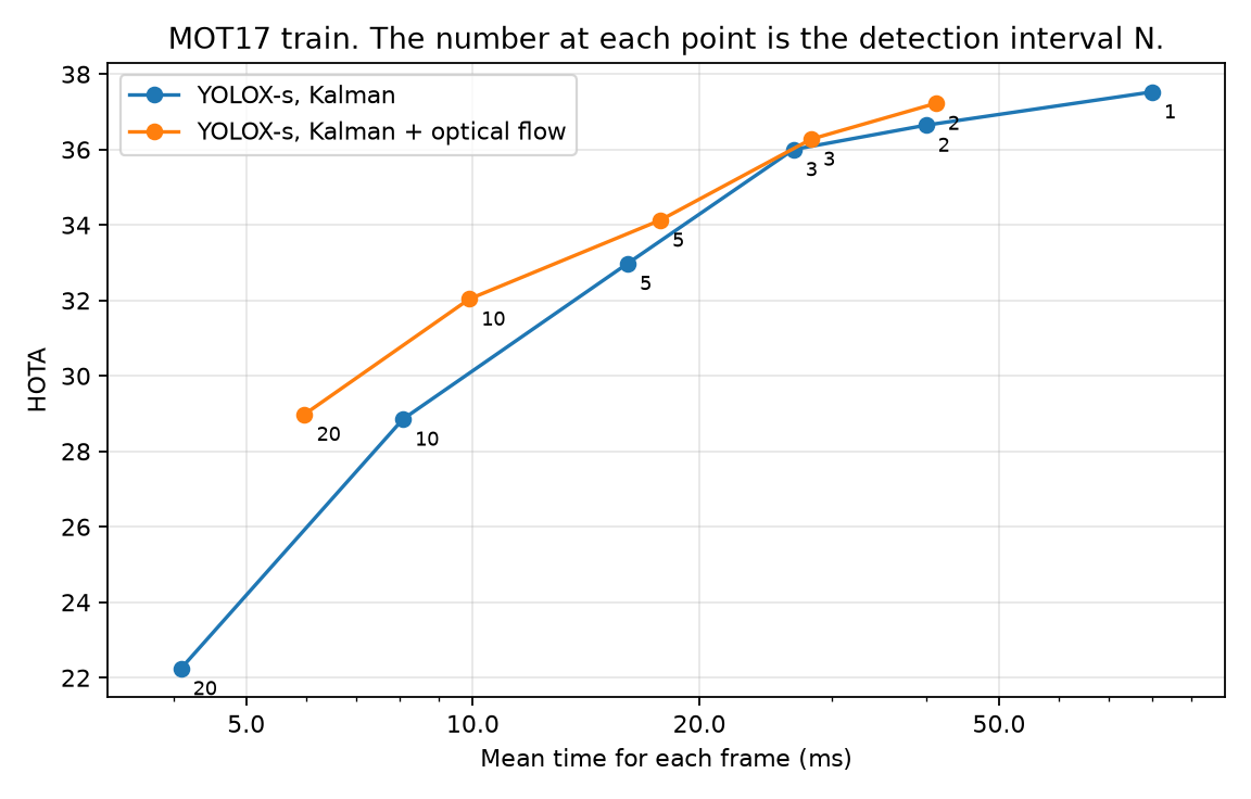
<p>Between detector runs, the tracker is guessing. It assumes each person keeps moving the way they were. I added optical flow, which follows small patches of the image from one frame to the next, and gave that motion to the tracker as a measurement.</p>
<p><img alt="HOTA against mean frame time, with and without optical flow. The line with optical flow is higher, and the gap grows at long intervals." src="/img/leantrack-interval.png" /></p>
<p>It costs less than 2 ms a frame. The gain grows with the interval: 0.3 points at every 3rd frame, 3.2 points at every 10th, 6.7 points at every 20th. It also cut identity switches by a third to a half. With flow, detecting every 10th frame is almost as good as detecting every 5th frame without it.</p>
<h2>The real problem: a live stream</h2>
<p>Everything above processes every frame and ignores the clock. So I simulated one. Frames arrive at the camera's rate, and an output only counts if it is ready before the next frame arrives.</p>
<p>I compared three loops:</p>
<ul>
<li><strong>Blocking.</strong> Wait for the detector, then take the newest frame. Frames in between are dropped.</li>
<li><strong>Background.</strong> The detector runs in its own thread. Every frame gets an output from the tracker and optical flow. When a detector result arrives it is a few frames old, so optical flow moves those boxes forward to the current frame before the tracker uses them.</li>
<li><strong>Background, no correction.</strong> The same, but the stale boxes are used as they are.</li>
</ul>
<table>
<thead>
<tr>
<th>Loop</th>
<th style="text-align: right;">Mean output latency</th>
<th style="text-align: right;">HOTA</th>
</tr>
</thead>
<tbody>
<tr>
<td>Blocking</td>
<td style="text-align: right;">101.4 ms</td>
<td style="text-align: right;">32.9</td>
</tr>
<tr>
<td>Background</td>
<td style="text-align: right;">5.1 ms</td>
<td style="text-align: right;">34.5</td>
</tr>
<tr>
<td>Background, no correction</td>
<td style="text-align: right;">2.8 ms</td>
<td style="text-align: right;">31.6</td>
</tr>
</tbody>
</table>
<p>The background loop answers about 20 times sooner (101.4 / 5.1 = 19.9) <strong>and</strong> scores 1.6 points higher. It is faster and better, which does not happen often.</p>
<p>The third row is the part I would have got wrong without measuring. A detection that arrives three frames late describes where people were three frames ago. Use it as it is and the score drops 2.9 points, below even the blocking loop. Moving the late boxes forward with optical flow is what makes the background design work.</p>
<h2>Two results I did not expect</h2>
<p><strong>The biggest model was not the best one.</strong> Offline, the larger YOLOX-m beats YOLOX-s, 40.0 to 37.5. On the live stream, in the background loop, it loses: 33.0 to 34.5. Its results arrive five frames old instead of three, and a better answer about the distant past is worth less than a decent answer about the recent past.</p>
<p><strong>A faster model beat a smarter schedule.</strong> I quantized YOLOX-s to 8-bit integers. That made it 2.8 times faster and cost 1.0 point offline. On the live stream it now fit inside one frame period, and a plain blocking loop with the quantized model scored 36.4, which is 1.9 points better than my careful background loop with the original model. All the scheduling work was worth less than making the detector fast enough to not need it.</p>
<h2>What did not work</h2>
<p>These are in the repository, because they changed the design.</p>
<p><strong>Triggering the detector when the tracker looks unsure.</strong> This seemed like the smart version of a fixed interval. I built two uncertainty signals, and they really do predict a bad box: when flow reliability was low, the box was wrong 78% of the time, against 16% when it was high. But running the detector at those moments did not fix the box. The trigger landed within half a point of a fixed interval, or below it. My guess is that low reliability often means the person is hidden, and a detector cannot see a hidden person either. I did not test that.</p>
<p><strong>Predicting which boxes are wrong.</strong> A small model on eight features reached an AUC of 0.73. One of those features alone reached 0.71. And its probabilities were off on scenes with a moving camera, so filtering on them made the score worse.</p>
<p><strong>The background loop for a fast detector.</strong> If the detector already fits in the frame period, moving it to the background just makes its answer one frame late. A blocking loop was 0.6 points better. I added a frame budget for this: wait for the detector only if it is expected to finish in time.</p>
<h2>One more thing: getting a lost person back</h2>
<p>When someone walks behind a pole, the tracker loses them. When they come out, do they get their old identity back?</p>
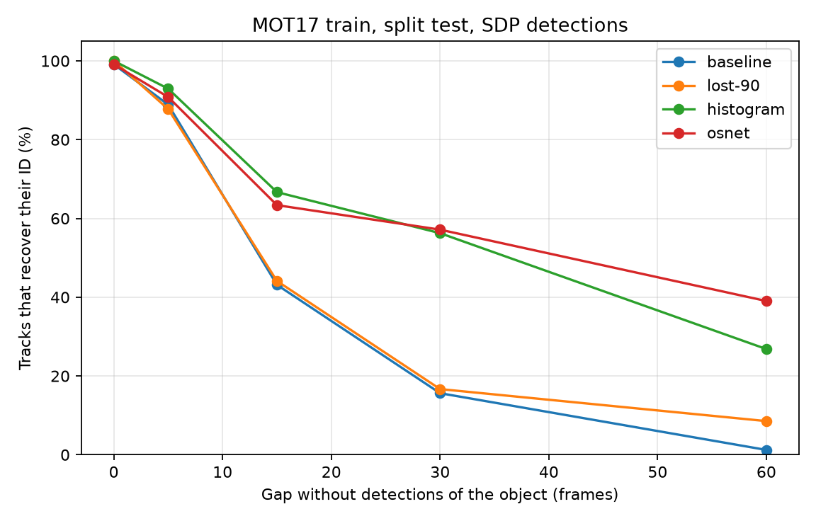
<p><img alt="Share of tracks that recover against the length of the gap, for four methods. The two appearance methods stay far above the two without appearance." src="/img/leantrack-occlusion.png" /></p>
<p>With position alone, 16% of tracks recovered after a 30-frame gap. Comparing appearance as well raised that to 57%. The surprise was how little was needed: a plain color histogram matched a neural re-identification network for gaps up to 30 frames, at a small fraction of the cost (0.07 ms a box against 1.6 ms). The network only pulled ahead on longer gaps.</p>
<p>And then the honest part: on the standard benchmark with strong detections, this changed the overall score by less than 0.1. The capability is real and the benchmark does not reward it.</p>
<h2>What I took from this</h2>
<ul>
<li><strong>Do not wait for a slow detector.</strong> Run it in the background and keep the tracks moving with optical flow.</li>
<li><strong>Correct late results.</strong> A stale detection used as fresh is worse than no background thread at all.</li>
<li><strong>Make the model faster before you make the schedule smarter.</strong> Quantization beat everything else I tried.</li>
<li><strong>Choose the model for the stream, not for the leaderboard.</strong> The best offline model was not the best live one.</li>
<li><strong>Keep the results that failed.</strong> Half of what I expected to work did not, and that is the more useful half.</li>
</ul>
<h2>Limits</h2>
<p>One laptop CPU, one run per configuration, no GPU and no small device. The live stream experiments use a simulated clock with measured timings, not a real camera. Changing the detector timing alone moves HOTA by about 0.7 on a live stream, so smaller differences between two live configurations are noise.</p>
<p>The code, every table, and eight short design records are in the <a href="https://github.com/yash-bitla/leantrack">repository</a>.</p></content>
  </entry>
  
  <entry>
    <title>Your RAG search may not need a reranker. Here is how I checked mine.</title>
    <link href="https://yashbitla.com/blog/testing-hybrid-search-advice/"/>
    <id>https://yashbitla.com/blog/testing-hybrid-search-advice/</id>
    <updated>2026-10-08T00:00:00Z</updated>
    <summary>I built a search engine in stages and measured each one on two datasets. Rank fusion did not beat dense retrieval, and neither reranker was worth its cost.</summary>
    <content type="html"><p>If you ask how to build good search for a RAG system, you get the same recipe almost everywhere: combine keyword search with vector search, fuse the two with reciprocal rank fusion, then put a reranker on top.</p>
<p>I wanted to know how much each step is worth. So I built the pipeline one stage at a time and measured every stage against the one before it. On the two datasets I used, about half of the recipe held up.</p>
<p>The code and every number in this post are in <a href="https://github.com/yash-bitla/hybrid-retrieval-engine">hybrid-retrieval-engine</a>.</p>
<h2>The setup</h2>
<p>I used two datasets from the <a href="https://github.com/beir-cellar/beir">BEIR</a> benchmark:</p>
<ul>
<li><strong>SciFact</strong>: 5,183 paper abstracts and 300 scientific claims to match against them.</li>
<li><strong>FiQA</strong>: 57,638 finance forum answers and 648 questions.</li>
</ul>
<p>The quality metric is nDCG@10. It runs from 0 to 1, and it is higher when the right documents are nearer the top of the first ten results.</p>
<p>I set three rules before I looked at any result:</p>
<ol>
<li><strong>Tune on training queries, test once.</strong> Anything with a knob was tuned on the training split. The test queries were used one time, for the final tables.</li>
<li><strong>Compare with a paired test.</strong> With 300 queries, the confidence interval on nDCG@10 is about ±0.045. Two retrievers that differ by 0.02 have overlapping intervals, but they answer the same queries, so I bootstrap the per-query difference instead. If that interval excludes zero, the difference is real.</li>
<li><strong>Check against published numbers.</strong> My BM25 scores 0.660 on SciFact and 0.236 on FiQA. The BEIR paper reports 0.665 and 0.236. If those had not matched, nothing after them would mean much.</li>
</ol>
<h2>Dense retrieval beat BM25. No surprise.</h2>
<p>BM25 is my own implementation: an inverted index that matches words. Dense retrieval uses a small embedding model (<code>bge-small-en-v1.5</code>) and matches by meaning.</p>
<table>
<thead>
<tr>
<th>Retriever</th>
<th style="text-align: right;">SciFact nDCG@10</th>
<th style="text-align: right;">FiQA nDCG@10</th>
<th style="text-align: right;">Latency (P50)</th>
</tr>
</thead>
<tbody>
<tr>
<td>BM25</td>
<td style="text-align: right;">0.660</td>
<td style="text-align: right;">0.236</td>
<td style="text-align: right;">under 1 ms</td>
</tr>
<tr>
<td>Dense</td>
<td style="text-align: right;">0.713</td>
<td style="text-align: right;">0.403</td>
<td style="text-align: right;">7 to 9 ms</td>
</tr>
</tbody>
</table>
<p>Dense is better on both, by 0.052 and 0.168, and both differences are significant. It is also slower, and almost all of that time is the model turning the query into a vector.</p>
<p>So far the recipe holds.</p>
<h2>Rank fusion did not beat dense retrieval</h2>
<p>This is the step everyone recommends. Reciprocal rank fusion (RRF) merges two rankings by position, so you do not need to make their scores comparable. It is simple and it needs no tuning.</p>
<p>It also did not help.</p>
<table>
<thead>
<tr>
<th>Compared with dense alone</th>
<th>SciFact</th>
<th>FiQA</th>
</tr>
</thead>
<tbody>
<tr>
<td>Hybrid with RRF</td>
<td>-0.009 (not significant)</td>
<td><strong>-0.054 (significant)</strong></td>
</tr>
<tr>
<td>Hybrid with a tuned weight</td>
<td>+0.018 (significant)</td>
<td>+0.009 (significant)</td>
</tr>
</tbody>
</table>
<p>On SciFact, RRF was no better than dense. On FiQA it was clearly worse.</p>
<p>The reason is that RRF gives both retrievers an equal vote. On FiQA, BM25 is far behind dense (0.236 against 0.403), so half of the vote comes from a much weaker system, and it pulls good results down.</p>
<p>A weighted fusion fixes this. I normalized each retriever's scores, then tried 11 weights on the training queries. The best mix was 70% dense on SciFact and 80% dense on FiQA. That version beat dense on both datasets.</p>
<p>But look at the size of the win: 0.018 and 0.009. It is real, and it is small. Hybrid search was not the big jump I expected. What it did improve on SciFact was recall: the share of relevant documents in the top 100 went from 94.2% to 96.8%.</p>
<h2>Neither reranker was worth its cost</h2>
<p>A reranker is a slower model that reads the query and each candidate together and rescores them. I tested two cross-encoders on SciFact, a small one (23M parameters) and a larger one (278M), each at four depths: rerank the top 10, 20, 50, or 100.</p>
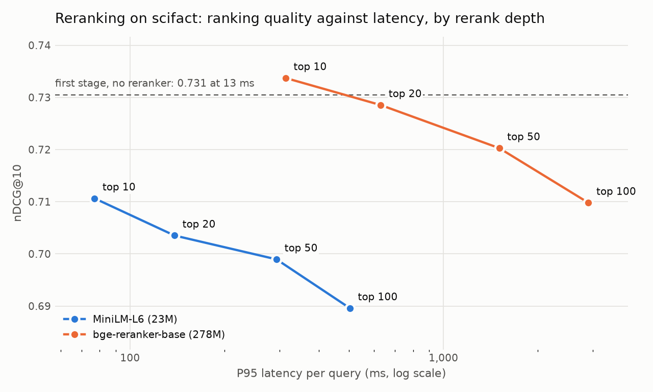
<p><img alt="nDCG@10 against P95 latency for two rerankers at four depths. Both lines fall as depth grows." src="/img/scifact-rerank.png" /></p>
<p>The dashed line is the pipeline with no reranker: 0.731 nDCG@10. The chart plots P95 latency, and the table below gives the median.</p>
<table>
<thead>
<tr>
<th>Reranker</th>
<th style="text-align: right;">Depth</th>
<th style="text-align: right;">nDCG@10</th>
<th>Change</th>
<th style="text-align: right;">Latency (P50)</th>
</tr>
</thead>
<tbody>
<tr>
<td>None</td>
<td style="text-align: right;"></td>
<td style="text-align: right;">0.731</td>
<td></td>
<td style="text-align: right;">11 ms</td>
</tr>
<tr>
<td>Small</td>
<td style="text-align: right;">10</td>
<td style="text-align: right;">0.711</td>
<td>-0.020</td>
<td style="text-align: right;">62 ms</td>
</tr>
<tr>
<td>Small</td>
<td style="text-align: right;">100</td>
<td style="text-align: right;">0.690</td>
<td>-0.041 (significant)</td>
<td style="text-align: right;">443 ms</td>
</tr>
<tr>
<td>Large</td>
<td style="text-align: right;">10</td>
<td style="text-align: right;">0.734</td>
<td>+0.003 (not significant)</td>
<td style="text-align: right;">312 ms</td>
</tr>
<tr>
<td>Large</td>
<td style="text-align: right;">100</td>
<td style="text-align: right;">0.710</td>
<td>-0.021</td>
<td style="text-align: right;">2,635 ms</td>
</tr>
</tbody>
</table>
<p>The small model made the ranking worse. The large one never moved it by a significant amount, and its best result cost 312 ms against 11 ms. That is 28 times the latency for nothing I could measure.</p>
<p>The part that surprised me most is the slope. Both lines go <strong>down</strong> as the reranker sees more candidates. The first stage already had 96.8% of the relevant documents in its top 100, so better documents were there to promote. The rerankers promoted the wrong ones.</p>
<p>My best guess is domain mismatch. Both rerankers are general-purpose models, and SciFact queries are scientific claims. I did not test that explanation, and I only ran the rerankers on one dataset, so treat this as one data point and not a law. It is still a useful one: a reranker is a hypothesis to test on your own data, not a default.</p>
<h2>The two speed-ups, and why only one mattered</h2>
<p><strong>Pruning BM25.</strong> A plain BM25 search reads every index entry for every query word. MaxScore, an algorithm from 1995, skips documents that cannot reach the top ten, and it returns exactly the same results.</p>
<table>
<thead>
<tr>
<th style="text-align: right;">Documents</th>
<th style="text-align: right;">Plain (P50)</th>
<th style="text-align: right;">MaxScore (P50)</th>
<th style="text-align: right;">Speed-up</th>
</tr>
</thead>
<tbody>
<tr>
<td style="text-align: right;">5,183</td>
<td style="text-align: right;">0.10 ms</td>
<td style="text-align: right;">0.04 ms</td>
<td style="text-align: right;">2.5x</td>
</tr>
<tr>
<td style="text-align: right;">57,638</td>
<td style="text-align: right;">0.76 ms</td>
<td style="text-align: right;">0.26 ms</td>
<td style="text-align: right;">2.9x</td>
</tr>
<tr>
<td style="text-align: right;">522,931</td>
<td style="text-align: right;">4.30 ms</td>
<td style="text-align: right;">0.45 ms</td>
<td style="text-align: right;">9.6x</td>
</tr>
</tbody>
</table>
<p>The gain grows with the corpus, and on the largest one MaxScore read only 5% of the index entries. I also ran the same compiled code with pruning switched off, and it was <em>slower</em> than the plain NumPy version. So the win comes from the algorithm and not from the compiler.</p>
<p><strong>Approximate vector search.</strong> HNSW is the index behind most vector databases. On FiQA it found 99.0% of the exact results and was 4.5 times faster than checking every vector (0.29 ms against 1.33 ms).</p>
<p>It also made almost no difference. Encoding the query takes 6.46 ms. So a full query went from 6.46 + 1.33 = 7.79 ms to 6.46 + 0.29 = 6.75 ms, which is 13% faster, in exchange for a longer build, more memory, and a small loss in recall. At 57,000 documents, a matrix multiplication is fine. By my estimate the index starts to matter somewhere near 280,000 documents, where exact search would cost as much as the encoder.</p>
<h2>What I would tell someone building search</h2>
<p>On these two datasets:</p>
<ul>
<li><strong>Start with dense retrieval.</strong> It was the largest single gain.</li>
<li><strong>Do not assume fusion helps.</strong> RRF with a weak partner hurt. If you fuse, tune the weight on held-out queries.</li>
<li><strong>Measure a reranker before you ship it.</strong> Mine cost 28 to 240 times the latency and gave nothing back.</li>
<li><strong>Find your real bottleneck first.</strong> I could have spent a week on a vector index to save one millisecond out of eight.</li>
</ul>
<p>And two things about method that mattered more than any single result:</p>
<ul>
<li><strong>Use a paired test.</strong> Without it, every comparison in this post would have read as "the intervals overlap, so who knows".</li>
<li><strong>Report the result you did not expect.</strong> I started this project expecting to show that hybrid search with a reranker wins. The honest version is more useful.</li>
</ul>
<h2>Limits</h2>
<p>Two datasets, one embedding model, two rerankers, and one laptop. The reranker result is from SciFact only. Latency ratios should transfer to other hardware better than the absolute numbers do. I would not be surprised if a domain-tuned reranker, or a different corpus, changed some of these conclusions, and that is the point: these are things to measure, not things to assume.</p>
<p>Everything here is reproducible from the <a href="https://github.com/yash-bitla/hybrid-retrieval-engine">repository</a>. If you run it on your own data and get a different answer, I would like to hear about it.</p></content>
  </entry>
  
  <entry>
    <title>Everything I know about getting better, I learned from shonen anime</title>
    <link href="https://yashbitla.com/blog/what-shonen-anime-taught-me/"/>
    <id>https://yashbitla.com/blog/what-shonen-anime-taught-me/</id>
    <updated>2026-01-05T00:00:00Z</updated>
    <summary>I grew up on Naruto, One Piece and Dragon Ball Z, and I never stopped watching. Here is what a lifetime of training arcs did to how I work.</summary>
    <content type="html"><p>I grew up watching anime, and I never grew out of it. I still watch every week. I collect figures, mostly Pop Mart, and I have stopped pretending they are for anyone but me.</p>
<p>For a long time I thought of this as the unserious part of my life, the thing I did when I was not doing real work. I had it backwards. A lot of how I work, and most of how I think about getting good at something hard, came from these shows before it came from anywhere else.</p>
<p>Here is what stuck.</p>
<h2>Naruto: nobody is coming to pick you</h2>
<p>Naruto starts the series as the kid nobody wants on their team. He is loud, he is bad at the basics, and he announces that he will lead the village one day to people who are openly laughing at him.</p>
<p>What I took from it was not "believe in yourself". It was the smaller, more useful thing underneath: he keeps showing up after it stops being fun. And the show is honest that talent is real. There are characters who are simply born better. The answer it gives is not that hard work beats talent. It is that hard work is the only part you control, so that is where you put your attention.</p>
<p>I think about that whenever I am the least experienced person in a room, which, early in a career, is most rooms.</p>
<h2>Dragon Ball Z: the ceiling is not where you think it is</h2>
<p>Dragon Ball Z has one idea and it repeats it for hundreds of episodes: the limit you just hit is not the limit.</p>
<p>Every arc, someone reaches a level that was supposed to be impossible, and then it becomes the new floor. As a kid, that was just exciting. As an adult, it is the most accurate description I know of how skill feels from the inside. The thing that seemed out of reach a year ago is now the thing you do without thinking, and you have forgotten that it was ever hard.</p>
<p>It also gave me Vegeta, which matters. He is the proud one who is always second, and he keeps training anyway. Most of us are Vegeta far more often than we are Goku. The show treats that as a respectable way to live.</p>
<h2>One Piece: long things are allowed to be long</h2>
<p>One Piece has been running since before I could read properly, and it is still going. It should not work. No story should be able to hold together for that long.</p>
<p>It works because the destination was never the point. The crew is. Each island is its own complete story, and the people on the ship get a little closer every time.</p>
<p>This is the show that taught me patience with long projects. Not every week has to end in a finale. Some weeks you are just sailing, and the sailing is the work. It also taught me that who you build with matters more than what you are building. I would take a good crew on a hard problem over a great problem on my own.</p>
<h2>Solo Leveling: the boring part is the system</h2>
<p>Solo Leveling looks like a power fantasy, and it is one. But the part I like is how it starts. The weakest hunter in the country gets a daily quest: push-ups, sit-ups, squats, and a run. Every day. Miss it and there is a penalty.</p>
<p>That is the whole secret, wrapped in a story about monsters. He does not get strong in the fights. He gets strong in the daily quest, and the fights are just where it shows.</p>
<p>It is the least glamorous lesson on this list and probably the truest. Almost everything I am decent at came from some small, repeated, slightly boring thing I did for much longer than felt reasonable.</p>
<h2>Demon Slayer: be good at it and be kind</h2>
<p>Tanjiro is one of the strongest characters in his world, and the thing everyone notices about him is that he is gentle. He trains until he breaks, and he still stops to feel sorry for the thing he just defeated.</p>
<p>I like that the show refuses to make these opposites. You do not have to pick between being excellent and being decent to people. The best people I have worked with were both, and it never seemed to cost them anything.</p>
<h2>Jujutsu Kaisen: strength has a bill</h2>
<p>And then there is Jujutsu Kaisen, which is the show I watch now, as an adult, and it is the one that complicates all of the above.</p>
<p>Here, getting stronger costs something, and the cost is real. The strongest character in the series is also the most alone. It is a shonen that has noticed what the genre usually skips: that the training arc takes things from you too.</p>
<p>I do not have a neat lesson from this one. I just think it is the right show to watch after you have absorbed all the others. Work hard, yes. Find your limit and go past it, yes. And then look up now and then and check what it is costing you.</p>
<h2>Why I still watch</h2>
<p>People sometimes ask, kindly, whether I am a bit old for this. I do not think you age out of it. The shows I loved at ten are still about the same things I care about now: getting better, not quitting, and looking after the people next to you. I just understand more of it.</p>
<p>The figures on my desk are not nostalgia. They are closer to a reminder. Do the daily quest. The ceiling is not where you think it is. Find a good crew.</p>
<p>And when it stops being fun, show up anyway.</p></content>
  </entry>
  
</feed>